Last time I argued that your data layout is your program, because the machine reads memory in 64 byte cache lines whether you asked for 64 bytes or 4. That post was about the CPU doing something less than you expected: it can only fetch whole lines, so a lot of what it fetches is wasted.
This one is about the CPU doing something considerably stranger. It runs your code before it knows whether it should.
Here’s the shape of what’s coming. I have an array of values and I want to count how many are above a threshold. I will not change the array, the count, the algorithm or the compiler flags. I will change the order of the elements, and the program will get twelve times faster.
for &value in values {
    if value > threshold {
        count += 1;
    }
}
That’s the whole program. There is nowhere for twelve times to hide.
The machine is guessing#
Your CPU does not execute one instruction at a time. It’s a pipeline: while one instruction is being executed, the next is being decoded, and the one after that is being fetched. On a modern core there are well over a dozen stages, and a hundred-odd instructions can be in flight at once. That parallelism is most of where modern performance comes from.
Now look at that if again, and notice the problem it creates. To keep the pipeline full, the CPU needs to
know which instruction comes next. But which instruction comes next depends on the comparison, and the
comparison hasn’t finished yet. The honest thing to do would be to stop and wait.
Modern CPUs are not honest. They guess.
The CPU predicts which way the branch will go, and then carries on fetching, decoding and executing down the guessed path as if it knew. If the guess was right, nothing was lost and the pipeline never stalled. If the guess was wrong, every instruction speculatively started behind that branch has to be thrown away, and the pipeline refilled from the correct address.
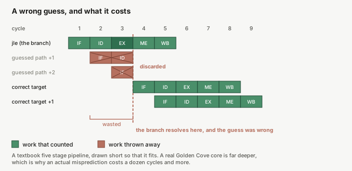
So a branch costs nothing when it is predicted correctly, and quite a lot when it isn’t. Which turns the interesting question into: how good is the guess?
The predictor is far cleverer than “assume the same as last time”. Modern designs keep a history of recent branch outcomes and use it to index tables of counters, so they can learn patterns rather than just tendencies. If you want the full lineage, the Wikipedia article walks from two-bit saturating counters through two-level adaptive predictors to the perceptron and TAGE designs in current silicon. What matters here is only the consequence: the predictor learns patterns, so its accuracy depends on whether your data has any.
How good is the guess?#
Let’s find out, by giving it data with a known amount of pattern in it.
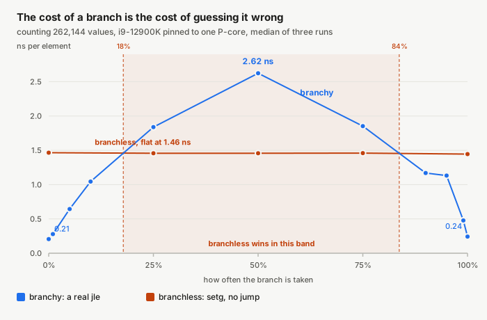
I generate an array where exactly some fraction of values sit above the threshold, and I shuffle it. At 0% the branch is never taken. At 100% it’s always taken. At 50% it’s a coin flip and there is nothing to learn. Then I count, and sweep that fraction from one end to the other.1
| taken | ns per element | mispredictions per element |
|---|---|---|
| 0% | 0.21 | 0.0000 |
| 1% | 0.28 | 0.0122 |
| 5% | 0.64 | 0.0793 |
| 10% | 1.04 | 0.1581 |
| 25% | 1.84 | 0.3267 |
| 50% | 2.62 | 0.4922 |
| 75% | 1.85 | 0.3221 |
| 90% | 1.17 | 0.1124 |
| 99% | 0.48 | 0.0100 |
| 100% | 0.24 | 0.0000 |
The same loop, over the same amount of data, doing the same amount of arithmetic, varies by a factor of more than twelve depending only on how predictable the branch is. At the extremes the predictor is right essentially always and the branch is free. In the middle it is guessing, and it is paying for it.
Two details in that table I find genuinely interesting.
The first is that at 50% the predictor mispredicts on 0.4922 of elements. The theoretical ceiling for a fair coin is 0.5. Against genuinely random data, all that clever history-tracking machinery achieves almost exactly nothing, which is the correct and expected outcome, and it is nice to see the hardware admit it.
The second is more surprising. At 25% taken, the miss rate is 0.327. But a predictor that ignored everything and always guessed “not taken” would be wrong only 0.25 of the time. The predictor is doing worse than the dumbest possible static guess, because it keeps trying to learn a pattern from a stream that hasn’t got one, and every time it half-learns something the data betrays it.
The same data, sorted#
Now the demonstration this result is famous for. If you’ve been writing software for a while you have probably seen the Stack Overflow question about sorted arrays; here it is on my machine.
I take the 50% array, the worst case above, and I sort it. Sorting doesn’t remove any values or change the answer. It doesn’t reduce the amount of work. All it does is put all the failing values before all the passing ones, so the branch goes one way for the first half and the other way for the second half.
| instructions | cycles | mispredictions | ns per element | |
|---|---|---|---|---|
| shuffled | 25,299,640,875 | 54,969,135,044 | 2,064,036,642 | 2.62 |
| sorted | 25,225,816,451 | 4,623,526,949 | 59,525 | 0.22 |
The two runs execute the same number of instructions, to within a third of a percent. One of them takes 11.9 times longer than the other. The entire difference is in the third column: 2.06 billion mispredictions against 59 thousand. Sorted, the predictor is right 99.999% of the time, because “same as the last few thousand” is a pattern and patterns are exactly what it eats.
This is the part that I think is worth sitting with. We are used to reasoning about performance by counting operations. Here the operation count is identical and the running time is not, because the cost was never in the instructions. It was in whether the machine could see them coming.
What one wrong guess costs#
We can do better than “quite a lot”, because those two rows are a controlled experiment: same data, same instruction count, only the order differs. Everything that differs between them is mispredictions, so divide one difference by the other.
(54,969,135,044 - 4,623,526,949) cycles / (2,064,036,642 - 59,525) misses = 24.4 cycles24.4 cycles per misprediction, measured on this machine rather than looked up. The textbooks quote 10 to 20 cycles, so mine is a bit worse than the folklore figure, which is what you’d expect from a core this deep: the more stages you have in flight, the more work there is to throw away. It is also an effective cost that includes everything downstream of the flush, not just the pipeline refill.
At a hair under 5 GHz, 24.4 cycles is about 5 nanoseconds. Every single time it guesses wrong.
Not having a branch at all#
If a mispredicted branch is expensive, one obvious response is to not have a branch. You can usually write the same logic as arithmetic:
count += (value > threshold) as u64;The comparison still happens, but its result becomes a 0 or a 1 that is added unconditionally. There is
nothing to predict, because control flow never diverges. In the assembly the jle is replaced by a setg,
which parks the comparison’s result in a register:
xorl	%r8d, %r8d
cmpl	%edx, (%rdi,%rax)
setg	%r8b
addq	%r8, -8(%rsp)
Look back at the chart and you’ll find that version as the flat line. It costs 1.46 ns per element regardless of the data, because it genuinely does not care about the data. It is immune.
But look where the lines cross. The branchless version is not faster. It is steadier, and the difference matters:
- Between roughly 18% and 84% taken, the branch is unpredictable enough that branchless wins.
- Outside that band, the branchy version wins, and at the extremes it wins by a factor of seven.
So “avoid branches” is not the lesson. The lesson is that a predictable branch is nearly free and an unpredictable one costs about 24 cycles, and the arithmetic version buys you insurance against the second case by giving up the first. If your branch is predictable more than about 85% of the time, that insurance is a bad deal.2
A different kind of branch#
Everything so far has been one branch going one of two ways. There is a second kind, and if you write Python you are leaning on it every microsecond.
An indirect branch doesn’t choose between two targets, it chooses between many. The canonical example is a bytecode interpreter, whose entire job is a loop that reads an opcode and jumps to the code implementing it:
for &op in code {
    acc = match op {
        Op::Inc => acc.wrapping_add(1),
        Op::Dec => acc.wrapping_sub(1),
        Op::Double => acc.wrapping_mul(2),
        // ... eight opcodes in total
    };
}
The compiler turns that match into a jump table, and the dispatch becomes a single instruction that jumps
to a computed address:
movzbl	(%rdi,%rcx), %r9d      # load the opcode
movslq	(%rdx,%r9,4), %r9      # look up its address in the jump table
addq	%rdx, %r9
jmpq	*%r9                   # jump to it, one branch, eight possible targets
Predicting this is a harder problem. It isn’t “taken or not”, it’s “which of eight”, and the hardware needs a different structure to do it. So: how well does that work?
I built programs with a controlled amount of repetition. Every opcode in this bytecode is total and accumulator-neutral, so any sequence is a valid program, and every program I generate contains exactly the same number of each opcode. The only thing that changes between them is the order. Some repeat with a period of 8, some 1024, and one is shuffled with no repeating structure at all.
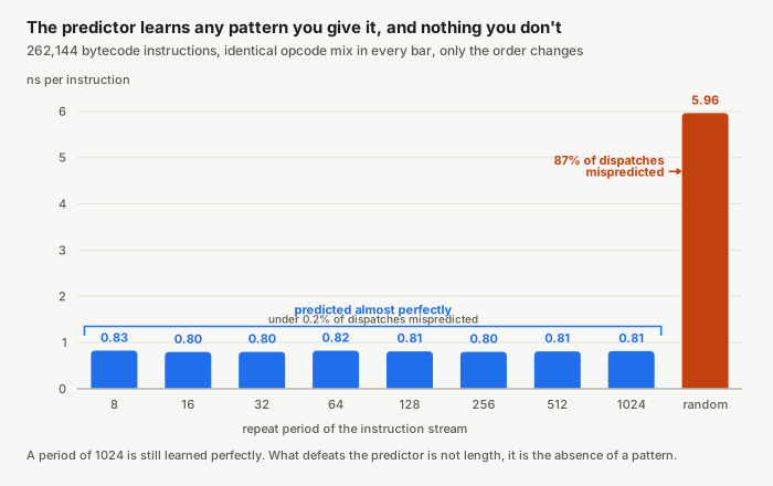
I expected to find the length at which the predictor gave up, and to be able to report it as the effective history length of the hardware. That is not what happened. Every repeating stream I threw at it, up to a period of 1024 instructions, was predicted essentially perfectly: fewer than 0.2% of dispatches mispredicted, around 0.8 ns per instruction throughout.
Then the random stream: 5.96 ns per instruction, and 87.3% of dispatches mispredicted. With eight equally likely targets, a predictor that learned nothing at all would miss 7 in 8, which is 87.5%. It got essentially nothing.
Running the same subtraction as before gives 29.7 cycles per indirect misprediction, a bit dearer than the 24.4 we measured for a conditional one, which makes sense: it isn’t enough to know the branch was wrong, the hardware also has to work out where it should have gone.
The shape of the answer is what I want you to take away. There is no gentle degradation and no cliff at some particular history length. There is a machine that learns any pattern you give it, and falls off a cliff only when there is no pattern to learn.
Don’t trust folklore#
Which brings me to the story I actually wanted to tell.
CPython’s interpreter loop is exactly the dispatch above, in C, with a hundred-odd opcodes instead of eight.
For years there was a well-known optimisation for interpreters written this way: replace the single switch
with a computed goto, duplicating the dispatch jump at the end of every opcode’s implementation. Same
work, but instead of one indirect branch that sees every opcode transition in the program, you get one per
opcode, each of which only ever sees the transitions that follow that opcode. The predictor has an easier
problem, and CPython’s own source notes the change was worth 15-20%.
That is a real optimisation. It is well explained, it is still in CPython today, and it worked.
Then, in 2015, Rohou, Swamy and Seznec published Branch Prediction and the Performance of Interpreters: Don’t Trust Folklore. They measured the misprediction rate of a switch-based CPython on successive generations of Intel hardware:
| CPU | mispredictions per 1000 instructions |
|---|---|
| Nehalem (2008) | 12.8 |
| Sandy Bridge (2011) | 3.5 |
| Haswell (2013) | 1.4 |
Nobody changed the interpreter. The predictors got better, and a problem that had justified a well-known optimisation quietly stopped being much of a problem. The advice was true when it was written. It just didn’t come with an expiry date, and the hardware it depended on kept moving underneath it.3
I opened the last post complaining that we teach performance as a list of rules, and that rules separated from their reasons decay into folklore. This is the cleanest example I know. “Switch dispatch mispredicts badly” was never a law of computing. It was an observation about a particular predictor at a particular time, and if that’s all you learned, you had no way of noticing when it expired. If you knew why it was true, you could have predicted its expiry yourself, from the same measurements I’ve just walked you through: the problem was always about how much pattern the hardware could learn, and the hardware got better at learning patterns.
That is the whole argument for understanding the machine underneath, and it isn’t about writing clever code. It’s that mechanisms age much more slowly than rules do.
Conclusion#
We started with a loop that got twelve times faster when I sorted its input without changing its output, and we’ve now seen why. The CPU keeps its pipeline full by guessing which way each branch will go, and it is extremely good at that when your data has a pattern and helpless when it doesn’t. We measured the cost of one wrong guess on this machine: 24.4 cycles for a conditional branch, 29.7 for an indirect one.
Along the way the numbers argued with me twice, which is the main reason to take them. The predictor turned out to do worse than a static guess on 25% random data. And the interpreter refused to show me the history limit I was looking for, because it learned every pattern I could construct and only broke on genuine noise.
The practical residue is small. Sorting your data to please the branch predictor is almost never worth it on its own, and going branchless is a real trade that only pays inside a band you’d have to measure to find. But if you now read “this branch is unpredictable” as “this costs about 5 nanoseconds every time”, you have the thing the rules were standing in for.
Next time I want to look at what happens when two cores touch the same cache line, and why the fix is sometimes to add padding you’ll never read.
The interpreter, the benchmarks and the instructions to reproduce all of this are in the repo for this blog. Your numbers will be different. That’s rather the point.
There is a trap here that I fell into first. The obvious way to write that counting loop doesn’t compile to a branch at all: LLVM vectorises it into
vpcmpgtdandvpaddq, a SIMD compare and add over eight values at a time, with no data dependent branch anywhere. Every number in this post would have been measuring nothing. The benchmarked version has an optimisation barrier inside the taken arm so that a realjlesurvives, and the branchless version carries the same barrier so the two differ only in the branch. If you take one habit from this series, let it be checking that the thing you’re measuring is the thing you think you’re measuring. ↩︎This is close to the figure Algorithmica quotes for the same trade, which is around 75% predictability on their hardware. Mine says 85%. Both are the same statement: it depends on your machine and your data, so measure it on yours. ↩︎
The thread that paper appeared in also carries a caveat worth repeating: this was an x86 result. ARM predictors of the era were considerably less sophisticated, so the same code could be folklore on one architecture and current on another, at the same moment. ↩︎